Context -Science- Climate Modelling –
Contents:
- What are Climate Models?
- How do Climate Models work?
- What are the inputs and outputs for a climate model?
- How accurate are climate model projections of temperature?
- What are the main limitations in climate modelling at the moment?
- What is the process for improving models
1. What are Climate Models
Climate models are key mathematical and computer based tools used to study complex climate dynamics and interactions. Following is a brief introduction presented from Skeptical Science:
Climate models are mathematical representations of the interactions between the atmosphere, oceans, land surface, ice – and the sun. This is clearly a very complex task, so models are built to estimate trends rather than events. For example, a climate model can tell you it will be cold in winter, but it can’t tell you what the temperature will be on a specific day – that’s weather forecasting. Climate trends are weather, averaged out over time – usually 30 years. Trends are important because they eliminate – or “smooth out” – single events that may be extreme, but quite rare….
Where models have been running for sufficient time, they have also been shown to make accurate predictions. For example, the eruption of Mt. Pinatubo allowed modellers to test the accuracy of models by feeding in the data about the eruption. The models successfully predicted the climatic response after the eruption. Models also correctly predicted other effects subsequently confirmed by observation, including greater warming in the Arctic and over land, greater warming at night, and stratospheric cooling.
The climate models, far from being melodramatic, may be conservative in the predictions they produce. Sea level rise is a good example (fig. 1).
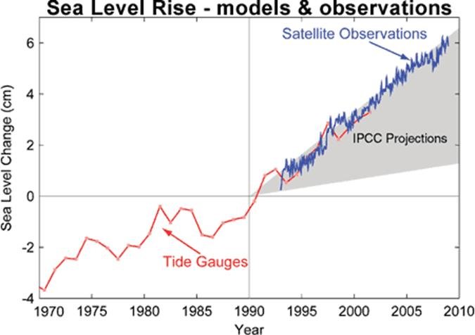
Fig. 1: Observed sea level rise since 1970 from tide gauge data (red) and satellite measurements (blue) compared to model projections for 1990-2010 from the IPCC Third Assessment Report (grey band). (Source: The Copenhagen Diagnosis, 2009)
Here, the models have understated the problem. In reality, observed sea level is tracking at the upper range of the model projections. There are other examples of models being too conservative, rather than alarmist as some portray them. All models have limits – uncertainties – for they are modelling complex systems. However, all models improve over time, and with increasing sources of real-world information such as satellites, the output of climate models can be constantly refined to increase their power and usefulness.
Climate models have already predicted many of the phenomena for which we now have empirical evidence. A 2019 study led by Zeke Hausfather (Hausfather et al. 2019) evaluated 17 global surface temperature projections from climate models in studies published between 1970 and 2007. The authors found “14 out of the 17 model projections indistinguishable from what actually occurred.”
2. How do Climate Models Work?
Carbon Brief offers a comprehensive and detailed account of what climate model are: Q&A: How do climate models work? – Carbon Brief how they work, how they are validated and how they are applied in climate science and reporting. It is certainly worth a look to obtain a good overview of this central tool of climate science prediction and climate policy making.
The remainder of this article comprises extracts from that article relating to the development of climate models, the types, how they work, the inputs, the limitations and further development:
What are the different types of climate models?
The earliest and most basic numerical climate models are Energy Balance Models (EBMs). EBMs do not simulate the climate, but instead consider the balance between the energy entering the Earth’s atmosphere from the sun and the heat released back out to space. The only climate variable they calculate is surface temperature. The simplest EBMs only require a few lines of code and can be run in a spreadsheet.
Many of these models are “zero-dimensional”, meaning they treat the Earth as a whole; essentially, as a single point. Others are 1D, such as those that also factor in the transfer of energy across different latitudes of the Earth’s surface (which is predominantly from the equator to the poles).
A step along from EBMs are Radiative Convective Models, which simulate the transfer of energy through the height of the atmosphere – for example, by convection as warm air rises. Radiative Convective Models can calculate the temperature and humidity of different layers of the atmosphere. These models are typically 1D – only considering energy transport up through the atmosphere – but they can also be 2D.
The next level up are General Circulation Models (GCMs), also called Global Climate Models, which simulate the physics of the climate itself. This means they capture the flows of air and water in the atmosphere and/or the oceans, as well as the transfer of heat.
Early GCMs only simulated one aspect of the Earth system – such as in “atmosphere-only” or “ocean-only” models – but they did this in three dimensions, incorporating many kilometres of height in the atmosphere or depth of the oceans in dozens of model layers.
More sophisticated “coupled” models have brought these different aspects together, linking together multiple models to provide a comprehensive representation of the climate system. Coupled atmosphere-ocean general circulation models (or “AOGCMs”) can simulate, for example, the exchange of heat and freshwater between the land and ocean surface and the air above.
The infographic below shows how modellers have gradually incorporated individual model components into global coupled models over recent decades.
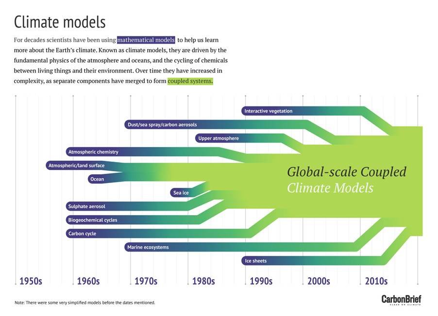
Graphic by Rosamund Pearce; based on the work of Dr Gavin Schmidt.
Over time, scientists have gradually added in other aspects of the Earth system to GCMs. These would have once been simulated in standalone models, such as land hydrology, sea ice and land ice.
The most recent subset of GCMs now incorporate biogeochemical cycles – the transfer of chemicals between living things and their environment – and how they interact with the climate system. These “Earth System Models” (ESMs) can simulate the carbon cycle, nitrogen cycle, atmospheric chemistry, ocean ecology and changes in vegetation and land use, which all affect how the climate responds to human-caused greenhouse gas emissions. They have vegetation that responds to temperature and rainfall and, in turn, changes uptake and release of carbon and other greenhouse gases to the atmosphere.
Prof Pete Smith, professor of soils & global change at the University of Aberdeen describes ESMs as “pimped” versions of GCMs:
“The GCMs were the models that were used maybe in the 1980s. So these were largely put together by the atmospheric physicists, so it’s all to do with energy and mass and water conservation, and it’s all the physics of moving those around. But they had a relatively limited representation of how the atmosphere then interacts with the ocean and the land surface. Whereas an ESM tries to incorporate those land interactions and those ocean interactions, so you could regard an ESM as a ‘pimped’ version of a GCM.”
There are also Regional Climate Models (“RCMs”) which do a similar job as GCMs, but for a limited area of the Earth. Because they cover a smaller area, RCMs can generally be run more quickly and at a higher resolution than GCMs. A model with a high resolution has smaller grid cells and therefore can produce climate information in greater detail for a specific area.
RCMs are one way of “downscaling” global climate information to a local scale. This means taking information provided by a GCM or coarse-scale observations and applying it to a specific area or region. Downscaling is covered in more detail under a later question.
Integrated Assessment Models:
Finally, a subset of climate modelling involves Integrated Assessment Models (IAMs). These add aspects of society to a simple climate model, simulating how population, economic growth and energy use affect – and interact with – the physical climate.
IAMs produce scenarios of how greenhouse gas emissions may vary in future. Scientists can then run these scenarios through ESMs to generate climate change projections – providing information that can be used to inform climate and energy policies around the world.
In climate research, IAMs are typically used to project future greenhouse gas emissions and the benefits and costs of policy options that could be implemented to tackle them. For example, they are used to estimate the social cost of carbon – the monetary value of the impact, both positive and negative, of every additional tonne of CO2 that is emitted.
3. What are the inputs and outputs for a climate model?
If the previous section looked at what is inside a climate model, this one focuses on what scientists put into a model and get out the other side.
The main inputs into models are the external factors that change the amount of the sun’s energy that is absorbed by the Earth, or how much is trapped by the atmosphere.
These external factors are called “forcings”. They include changes in the sun’s output, long-lived greenhouse gases – such as CO2, methane (CH4), nitrous oxides (N2O) and halocarbons – as well as tiny particles called aerosols that are emitted when burning fossil fuels, and from forest fires and volcanic eruptions. Aerosols reflect incoming sunlight and influence cloud formation.
Typically, all these individual forcings are run through a model either as a best estimate of past conditions or as part of future “emission scenarios”. These are potential pathways for the concentration of greenhouse gases in the atmosphere, based on how technology, energy and land use change over the centuries ahead.
Today, most model projections use one or more of the “Representative Concentration Pathways” (RCPs), which provide plausible descriptions of the future, based on socio-economic scenarios of how global society grows and develops. You can read more about the different pathways in this earlier Carbon Brief article.
Models also use estimates of past forcings to examine how the climate changed over the past 200, 1,000, or even 20,000 years. Past forcings are estimated using evidence of changes in the Earth’s orbit, historical greenhouse gas concentrations, past volcanic eruptions, changes in sunspot counts, and other records of the distant past.
Then there are climate model “control runs”, where radiative forcing is held constant for hundreds or thousands of years. This allows scientists to compare the modelled climate with and without changes in human or natural forcings, and assess how much “unforced” natural variability occurs.
What is CMIP?
With so many institutions developing and running climate models, there is a risk that each group approaches its modelling in a different way, reducing how comparable their results will be.
This is where the Coupled Model Intercomparison Project (“CMIP”) comes in. CMIP is a framework for climate model experiments, allowing scientists to analyse, validate and improve GCMs in a systematic way.
The “coupled” in the name means that all the climate models in the project are coupled atmosphere-ocean GCMs. The Met Office’s Dr Chris Jones explains the significance of the “intercomparison” part of the name:
“The idea of an intercomparison came from the fact that many years ago different modelling groups would have different models, but they would also set them up slightly differently, and they would run different numerical experiments with them. When you come to compare the results you’re never quite sure if the differences are because the models are different or because they were set up in a different way.”
So, CMIP was designed to be a way to bring into line all the climate model experiments that different modelling centres were doing.
Since its inception in 1995, CMIP has been through several generations and each iteration becomes more sophisticated in the experiments that are being designed. A new generation comes round every 5-6 years.
In its early years, CMIP experiments included, for example, modelling the impact of a 1% annual increase in atmospheric CO2 concentrations (as mentioned above). In later iterations, the experiments incorporated more detailed emissions scenarios, such as the Representative Concentration Pathways (“RCPs”).
Setting the models up in the same way and using the same inputs means that scientists know that the differences in the climate change projections coming out of the models is down to differences in the models themselves. This is the first step in trying to understand what is causing those differences.
How are climate models “parameterised” and tuned?
As mentioned above, scientists do not have a limitless supply of computing power at their disposal, and so it is necessary for models to divide up the Earth into grid cells to make the calculations more manageable.
This means that at every step of the model through time, it calculates the average climate of each grid cell. However, there are many processes in the climate system and on the Earth’s surface that occur on scales within a single cell.
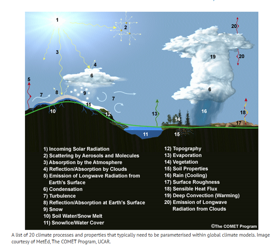
.. The graphic below shows some of the processes that are typically parameterised in models.
Parameterisations may also be used as a simplification where a climate process isn’t well understood. Parameterisations are one of the main sources of uncertainty in climate models.
…As most global models will contain parameterisation schemes, virtually all modelling centres undertake model tuning of some kind. A survey in 2014 (pdf) found that, in most cases, modellers tune their models to ensure that the long-term average state of the climate is accurate – including factors such as absolute temperatures, sea ice concentrations, surface albedo and sea ice extent.
…Essentially, scientists compare long-term statistics in the model output with observed climate data. Using statistical techniques, they then correct any biases in the model output to make sure it is consistent with current knowledge of the climate system.
Bias correction is often based on average climate information, Maraun notes, though more sophisticated approaches adjust extremes too.
4. How accurate are climate model projections of temperature?
In order to evaluate how well their models perform, scientists compare observations of the Earth’s climate with models’ future temperatures forecasts and historical temperatures “hindcasts”. Scientists can then assess the accuracy of temperature projections by looking at how individual climate models and the average of all models compare to observed warming.
If models do a good job of capturing the climate response in the past, researchers can be more confident that they will accurately respond to changes in the same factors in the future.
Comparing global air temperatures from the models to a combination of air temperatures and sea surface temperatures in the observations can create problems. To account for this, researchers have created what they call “blended fields” from climate models, which include sea surface temperatures of the oceans and surface air temperatures over land, in order to match what is actually measured in the observations.
These blended fields from models show slightly less warming than global surface air temperatures, as the air over the ocean warms faster than sea surface temperatures in recent years.
The longer period of model projections from 1880 through 2100 is shown in the figure below. It shows both the longer-term warming since the late 19th century and projections of future warming under a scenario of relatively rapid emissions reductions (called “RCP4.5”), with global temperatures reaching around 2.5C above pre-industrial levels by 2100 (and around 2C above the 1970-2000 baseline shown in the figure).
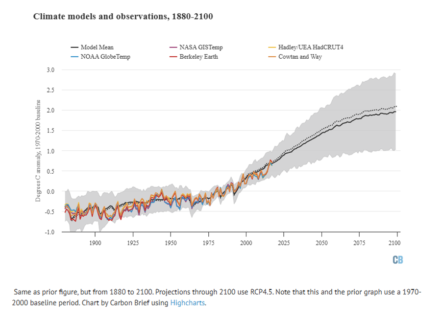
Projections of the climate from the mid-1800s onwards agree fairly well with observations. There are a few periods, such as the early 1900s, where the Earth was a bit cooler than models projected, or the 1940s, where observations were a bit warmer.
Overall, however, the strong correspondence between modelled and observed temperatures increases scientists’ confidence that models are accurately capturing both the factors driving climate change and the level of short-term natural variability in the Earth’s climate.
5. What are the main limitations in climate modelling at the moment?
Yet, despite models becoming increasingly complex and sophisticated, there are still aspects of the climate system that they struggle to capture as well as scientists would like.
Clouds
One of the main limitations of the climate models is how well they represent clouds.
Clouds are a constant thorn in the side of climate scientists. They cover around two-thirds of the Earth at any one time, yet individual clouds can form and disappear within minutes; they can both warm and cool the planet, depending on the type of cloud and the time of day; and scientists have no records of what clouds were like in the distant past, making it harder to ascertain if and how they have changed.
Instead, scientists use “parameterisations” (see above) that represent the average effects of convection over an individual grid cell. This means GCMs do not simulate individual storms and local high rainfall events, explains Dr Lizzie Kendon, senior climate extremes scientist at the Met Office Hadley Centre, to Carbon Brief
Double ITCZ
Related to the issue of clouds in global models is that of “double ITCZ”. The Intertropical Convergence Zone, or ITCZ, is a huge belt of low pressure that encircles the Earth near the equator. It governs the annual rainfall patterns of much of the tropics, making it a hugely important feature of the climate for billions of people.
Most GCMs show some degree of the double ITCZ issue, which causes them to simulate too much rainfall over much of the southern hemisphere tropics and sometimes insufficient rainfall over the equatorial Pacific.
The double ITCZ “is perhaps the most significant and most persistent bias in current climate models”, says Dr Baoqiang Xiang, a principal scientist at the Geophysical Fluid Dynamics Laboratory at the National Oceanic and Atmospheric Administration in the US.
Jet streams
Finally, another common issue in climate models is to do with the position of jet streams in the climate models. Jet streams are meandering rivers of high-speed winds flowing high up in the atmosphere. They can funnel weather systems west to east across the Earth.
As with the ITCZ, climate models recreate jet streams as a result of the fundamental physical equations contained in their code.
As a result, models do not always get it right on the paths that low-pressure weather patterns take – known as “storm tracks”. Storms are often too sluggish in models, says Woollings, and they do not get strong enough and they peter out too quickly.
6. What is the process for improving models?
The process of developing a climate model is a long-term task, which does not end once a model has been published. Most modelling centres will be updating and improving their models on a continuous cycle, with a development process where scientists spend a few years building the next version of their models.
Once ready, the new model version incorporating all the improvements can be released, says Dr Chris Jones from the Met Office Hadley Centre:
“It’s a bit like motor companies build the next model of a particular vehicle so they’ve made the same one for years, but then all of a sudden a new one comes out that they’ve been developing. We do the same with our climate models.”
At the beginning of each cycle, the climate being reproduced by the model is compared to a range of observations to identify the biggest issues, explains Dr Tim Woollings. He tells Carbon Brief:
“Once these are identified, attention usually turns to assessing the physical processes known to affect those areas and attempts are made to improve the representation of these processes [in the model].”
At the Met Office Hadley Centre, the development process involves multiple teams, or “Process Evaluation Groups”, looking to improve a different element of the model, explains Woollings:
“The Process Evaluation Groups are essentially taskforces which look after certain aspects of the model. They monitor the biases in their area as the model develops, and test new methods to reduce these. These groups meet regularly to discuss their area, and often contain members from the academic community as well as Met Office scientists.
The improvements that each group are working on are then brought together into the new model. Once complete, the model can start to be run in earnest, says Jones:
“At the end of a two- or three-year process, we have a new-generation model that we believe is better than the last one, and then we can start to use that to kind of go back to the scientific questions we’ve looked at before and see if we can answer them better.”
7. Recent Articles
- Climate science: Are we underestimating global warming? What if our climate models are wrong? | Vox – Sep 24
- Climate model biases in global monsoon: Insights from interhemispheric energy transport (phys.org) – Aug 24
– Jul 24- Albedo too high by about 5% – GIS melting faster than older model version – microphysical properties in warming world